This first part of an edited contribution to INMR by Riccardo Bonanno and Michele de Nigris of RSE in Italy discusses characterizing and understanding recurrent cable joint failures under heavy climatic and electrical stresses.
It also reviews research carried out to elucidate the phenomena at the base of the threat, assess vulnerability of a medium voltage cable network and its components and identify measures to increase resilience of power systems against weather extremes.

Underground Distribution Cables in the Italian Power System
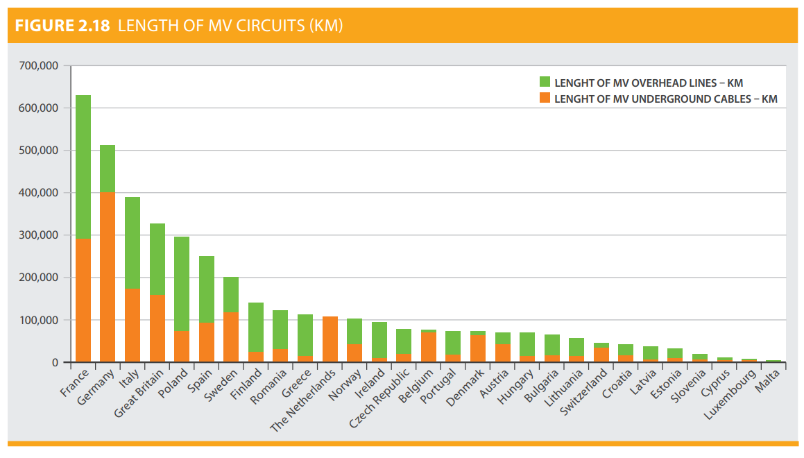
As shown in Fig. 1, underground cables represent the core of the distribution system across many countries within Europe. Among these, Italy, with its topography and geographic characteristics as well as high level of electrification, scores high in terms of overall line length (395,000 km) and MV distribution line density (1.3 km of lines per km2 of land). Initially used in major cities to enhance use of space, increase safety and reduce visual impact of overhead lines, application has progressively increased outside metropolitan areas. Main factors in this regard were intrinsic reliability and reduced vulnerability to contact with trees, heavy wind, wet snow, failure of structures and accidents due to bare conductors.
The Italian MV distribution system is laid underground for nearly 45% of its extension (total MV cables 175,000 km). In terms of technologies, oil or resin impregnated paper that was used widely until the end of the 1970s, has been progressively replaced by XLPE extruded insulation. In most cities, however, mixed technologies are the norm and 50 to 60% of old resin-insulated cable sections are connected to dry sections using transition joints.
Undergrounding MV distribution cable is a practice that has long been adopted. Solutions for cable jointing cover the entire technological panorama, from belted joints to resin joints, heat shrink joints or cold shrink types.
Heat and cold shrink joints are at present seen as the best technologies since they are rapid to install in the field and can be energized only 30 minutes after mounting. Cold shrink joints are currently the most widely used in cable works (whether new installation or repair) because they are modular. Based on pieces made in the factory under a supervised quality control program, they require only simple manipulation. They also significantly shorten outage time of a line, thus improving a system’s power quality parameters.
Reliability of MV Underground Cable Lines
Unfortunately, evolution in cables, joints and terminations has not always been accompanied by a significant increase in line reliability. In fact, it has been recognized that distribution system operators across Italy often observe significant increases in failure rates in their medium voltage underground cable networks. This appears most concentrated over the hottest period from May to October and especially so during persistent heat waves characterized by ambient temperatures well above historical values combined with lack of precipitation and high relative humidity. Indeed, these conditions can be a prerequisite to poor heat dissipation of highly stressed underground cables.
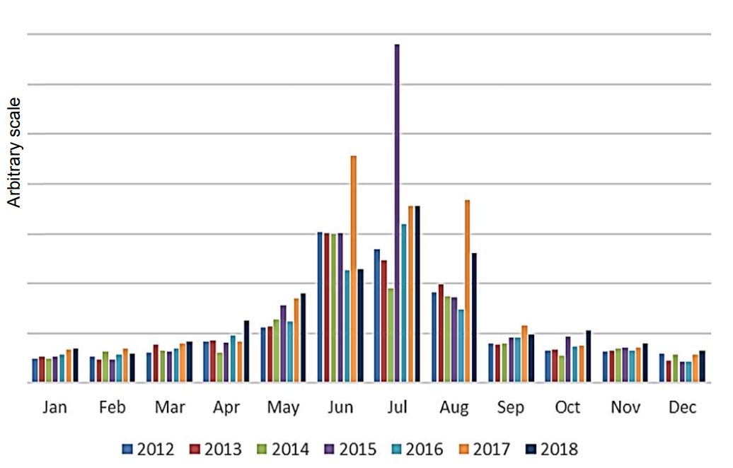
This situation is depicted in Fig. 2, which shows unexpected, non-accidental failure data for MV cable joints for the period 2012 to 2018, as reported by one Italian distribution system operator. The Y-axis is not numbered because the aim is to depict the trend. Failures occur more often in some years than others because of the variable frequency and duration of adverse conditions such as heat wave and low rainfall.
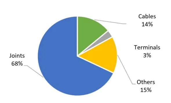
The first step of the analysis identified cable joints as the weakest point in the system. See Fig. 3, which shows the source of MV cable failures in Italy and indicates that about 70% of failures occur in cable joints, while only about 15% in the cable insulation. Understanding the reasons why cable joints appear to have poor service performance and related threats has therefore become a topic of different research projects. These look to consider external phenomena such as climate as well as intrinsic aspects of the cable system such as technology, installation method, maintenance, monitoring and operation.
The Threat: Heat Waves & Soil Dry-Out Phenomenon
Heat Waves
The World Meteorological Organization defines a heat wave as five or more consecutive days of sustained heat in which the daily maximum temperature is 5°C or more above average maximum temperature. The reference period for calculating this average is between 1961 and 1990. Some countries have established their own criteria to define a heat wave.
Heat waves are of particular interest to network operators because they can contribute to widespread failures due to the simultaneous presence of several fault-triggering factors, including:
• increase in soil temperature;
• increase in electrical load of cables;
• increase in thermal resistivity of the soil linked with reduction in relative humidity of terrain under these conditions (see soil dry-out below).
Soil Dry-Out
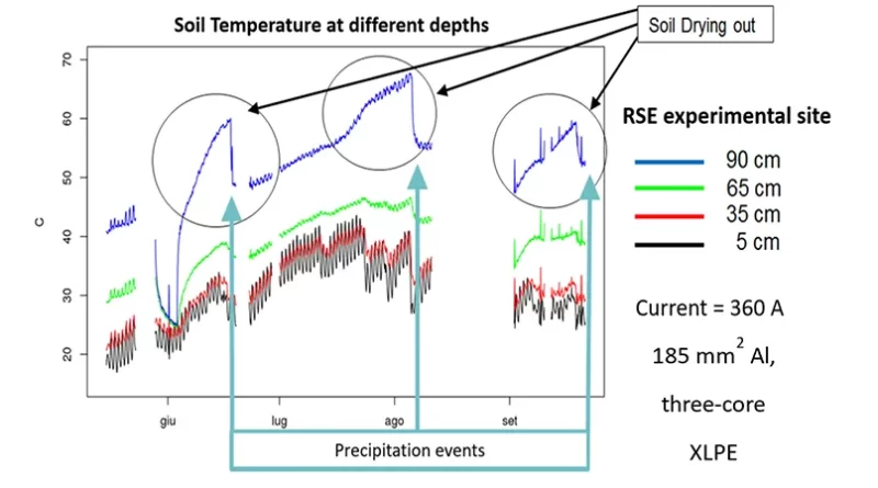
The phenomenon of ‘soil dry-out’ occurs in the presence of a major heat source in contact with the ground, such as a current-carrying cable of an underground power line that dissipates heat by the Joule effect (see Fig. 4). Temperatures reached by the cable under normal operating conditions can easily exceed 60°C in summer (Note: From a functionality point of view, maximum conductor temperature of paper insulated cables is 75°C while that of extruded cables is 90°C). At these temperatures, the heat dissipated by the cable can vaporize moisture in the soil. The moisture gradient generated causes steam flow through soil porosity toward colder areas, where it recondenses. The air filling the soil porosities in place of moisture, with its low thermal conductivity, then prevents dissipation of heat, leading to increased cable temperature, i.e. one of the greatest risks for accelerated ageing of cable insulation.
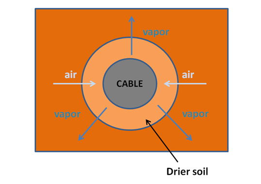
Fig. 5 shows the temperature time series at 4 different depths in the soil (5, 35, 65 and 90 cm) using a set-up aimed at studying and monitoring this phenomenon in the presence of a loaded cable. The period reported refers to the summer of 2010. The cable used in this experiment was a 185 mm2 Al, three-core XLPE. This figure highlights 3 periods in which the temperature of the deepest soil layer on which the cable is located has a pronounced growth ramp. In this situation, soil dry-out creates an overheating of the soil near the cable, as described above. Only significant precipitation events can stop this rise in temperature and re-establish it on lower values. The infiltration of water into the soil increases the thermal conductivity which therefore allows the cable to dissipate the accumulated heat again.


Setting Up Fault Prediction Model: Step 1 – Identification of Indicators
Power quality is a priority for the National Regulatory Authority for Energy, Networks, and the Environment (ARERA). Regulation in this field aims to motivate network operators to improve average power supply continuity, thus approaching European levels. Also to reduce the gap between Northern and Southern regions of Italy and protecting consumers through the provision of automatic compensation in the event of non-compliance with the standards set by the regulation. ARERA has obliged distribution system operators to elaborate plans aimed at increasing the resilience of the electricity networks under their responsibility, through the Resolution 646/2015/R/eel “Integrated text of the regulation output- basis of electricity distribution and metering services – 2016-2023 regulatory period” (Annex A, Integrated Text on Electrical Quality, TIQE). These plans must include investments as well as interventions aimed at reducing risk of faults and outages against threats.
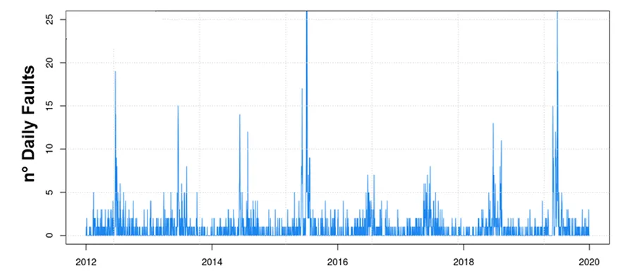
With the aim of setting up a fault rate prediction model for underground cables over an entire city (based on meteorological and load data), the first step consisted of identifying any correlation between possible influencing factors and the observed faults. The data forming the basis of this study were faults provided by the distribution company for Milan. The data was provided in tabular format and associated with different points in the city where faults were observed. The data was then aggregated to obtain daily number of faults for the city.
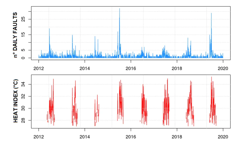
Fig. 6 shows daily faults from 2012 to 2019. It can be noticed that faults are also observed in other seasons besides summer, but they increase significantly in frequency during the summer period, often showing a first more significant peak at the beginning of the season (June) when the first summer heat waves occur. The exception is represented by the years 2015 and 2019 in which a more significant secondary peak could be observed corresponding to powerful heat waves that affected Italy during the month of July.
This behavior can be explained by the fact that at the beginning of the summer period with the first heat waves (not necessarily the strongest one) most vulnerable and aged joints are subject to faults and are progressively replaced. Hence, with the following heat waves, the network can better absorb the thermal stresses, unless a very powerful heat waves occurs, such as in 2015 and 2019.
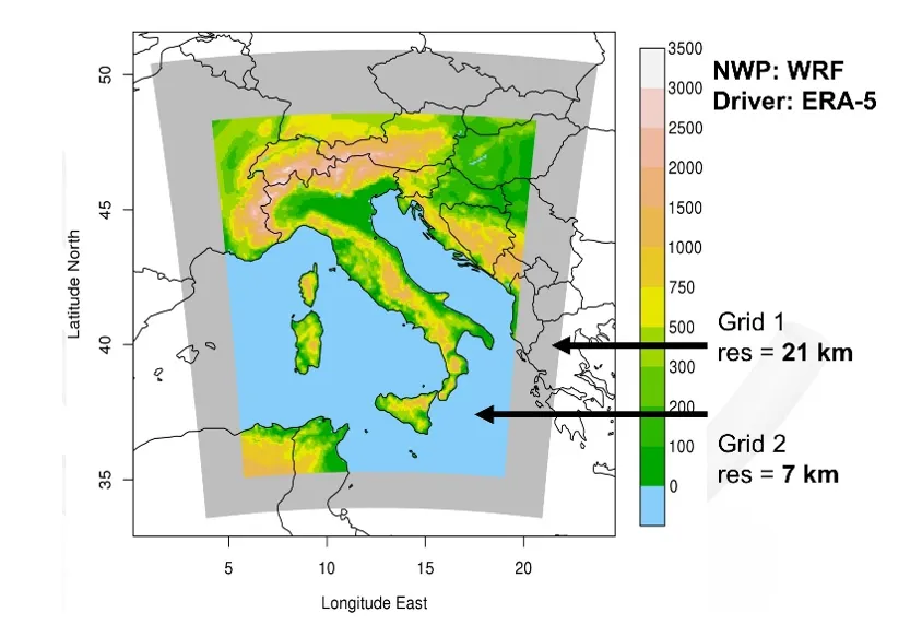
Meteorological variables derive from the meteorological reanalysis dataset MERIDA (MEteorological Reanalysis Italian Dataset, [7]), developed in RSE to respond to the increasing demand for high spatial and temporal resolution historical weather data, necessary for stakeholders in the electro-energy sector, so that they can implement adaptation strategies to safely operate the electricity system. MERIDA consists of a dynamical downscaling of the new European Centre for Medium-range Weather Forecasts (ECMWF) [8] global reanalysis ERA5 [9] using the Weather Research and Forecasting (WRF) model, which is configured to describe the typical weather conditions of Italy. The computational domain is defined using two grids with a spatial resolution of 21 km and 7 km respectively, with the internal grid centred over Italy as shown in Figure 7. The dataset has hourly temporal resolution and spans over 30 years, with 22 different meteorological variables computed at 40 different altitude levels and comprises 1,5*1012 records. The advantage in the availability of a meteorological reanalysis consists in the possibility of having a reconstruction of observations even in points of the domain where no observations are available from experimental meteorological stations. Moreover, this reanalysis provides data of soil temperature and moisture whose experimental availability is even more limited than atmospheric experimental data (i.e., temperature and precipitation).
Correlation Between Faults & 2m Temperature
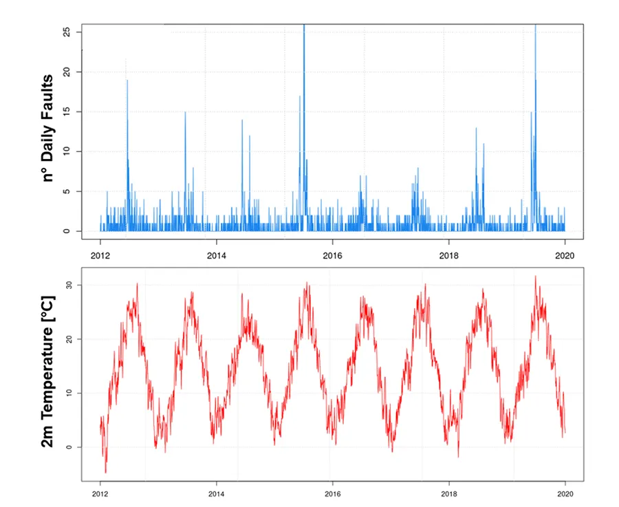
The first and most intuitive quantity to consider in the search of correlations is ambient temperature. Here, temperature at 2m height is considered from the MERIDA data set. Comparing fault time series for Milan Urban Area with 2m temperature (see Fig. 8), there is clear correlation between fault peaks and temperature peaks associated with summer heat waves. This indicates that one of the primary possible causes of significant increase in faults in the summer relates to heat waves.

Correlation Between Faults & Heat Index
A further variable that has been considered in analysis of correlations between faults and weather variables is the Heat Index, which is a meteorological indicator defined by NOAA (http://www.wpc.ncep.noaa.gov/html/heatindex_equation.shtml) to estimate the physiological discomfort caused by presence of high air temperature and humidity. The Heat Index is defined only for values of temperature higher than 27°C and for values of relative humidity (RH) higher than 40%. The key point to consider is that the higher the RH, the more difficulty a human body has dissipating the heat. This index can, therefore, be considered as a proxy for energy demand for cooling since it is closely linked to the physiological discomfort associated to high air temperature and humidity.
Fig. 9 shows the faults time series for Milan Urban Area correlated with the related Heat Index. Thresholds in temperatures and relative humidity, intrinsic to definition of the Heat Index, imply that for certain periods values are missing from the related time series.
Comparing the two trends, there is clear correlation between fault peaks and Heat Index peaks associated with summer heat waves. Often, the highest peaks of Heat Index in summer season do not correspond with the highest peaks of daily failures because the most extended failure events occur at the beginning of the summer season, when the weakest joints break down with occurrence of the first heat waves (which may not necessarily be the strongest).
Correlation Between Faults & Soil Temperature/Moisture
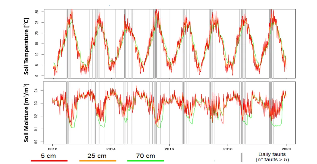
Another important driving factor is linked with the thermal condition of the soil in which the cables are laid down. In particular, soil temperature and moisture values are extracted in MERIDA for 3 soil depths: 5, 25, 70 cm. (It should be noted that MERIDA soil layers depths are different from the depths of the experimental set-up, as shown in Fig. 5).
In Fig. 10, in addition to the soil variables, daily faults recorded in Milan in the same period (vertical grey lines) are superimposed. Only days with daily faults higher than 5 are represented. It can be seen that periods of highest frequency of faults often correspond to periods with temperature peaks associated with heat waves and to periods with dry soil, especially in the deep layer (70 cm, green line), which is the one closest to the depth where the underground cables are usually located.
The soil type described by MERIDA derives from the FAO Soil Texture classification. Given the low resolution of the dataset, the soil type described in a certain pixel provides only an indicative and average characteristic of the soil in a given region. Moreover, corresponding to any urban area, the situation becomes more complex because soil type is seldom homogeneous and often interspersed with layers of asphalt, cement or built-up soil with mixed characteristics (i.e. heterogeneous mixture of natural soil and anthropic origin). Estimate of temperature and humidity provided by MERIDA dataset is therefore affected by some margin of uncertainty since assumed soil type may not coincide with actual existing type. Nonetheless, this can still be considered as the best estimate of these variables.
Correlation Between Faults & Daily Load
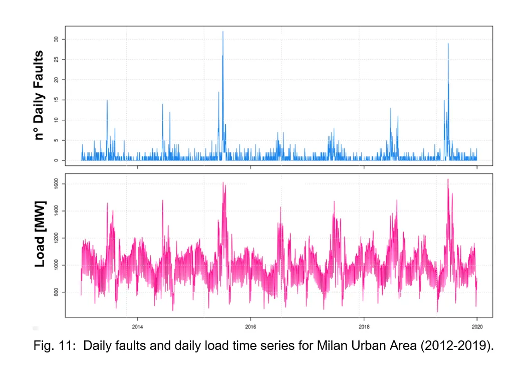
Finally, one of the most important parameters correlated to faults is the cable load. Daily load data for the city of Milan are represented in Fig. 11 together with the faults time series from 2012 to 2019. Looking at the load time series, a certain cyclicity on an annual scale can be noticed, in addition to the weekly cycle, with peaks in conjunction with winter and summer. The winter peak is abruptly interrupted in the period around Christmas, while the summer peak in conjunction with holidays in August.
A clear correlation between daily load and faults time series can be noticed. The greatest number of faults occurs in periods with most pronounced load fluctuations. Load peaks are obviously correlated with weather associated with heat waves because of the high load demand for cooling. Stress conditions on joints are therefore clearly linked both to the massive load in the underground distribution network and to high soil temperatures.
Correlation Between Faults & Temperature of Typical Current-Carrying Conductor
Together with estimates of temperature and soil moisture provided by the MERIDA dataset, a correlation with faults was also investigated considering an estimate of the temperature of a generic underground current-carrying conductor, subjected to stress conditions associated to high soil temperatures and low soil moisture, as typical of summer periods. For this purpose, the temperature model of the cable was considered, given the flowing current and the thermal resistivity of the soil in the presence of partial soil dry out, as described in the standard CEI EN 60287-1-1: 2001.
Tc=Ta+I2 R(T1+n(1+λ1 ) T2+n(1+λ1+λ2 )(T3+T4 ))+Wd (0.5T1+n(T2+T3+T4 )) (1)
where:
Ta : is the ambient temperature, namely the temperature in soil at the cable depth
I: current circulating in conductor
R : alternating current resistance of the conductor at its maximum operating temperature
Wd : dielectric loss per unit length for the insulating material around the conductor
λ1 : dielectric loss per unit length for the insulating material around the conductor
λ 2 : ratio of armouring losses to the total losses of conductors in that cable
T1 : Thermal resistance per core between conductor and sheath
T2 : Thermal resistance between sheath and armour
T3 : Thermal resistance of external serving
T4 : Thermal resistance of surrounding medium
The terms T3 and T4 depend on thermal conductivity of the soil which in turn, as already mentioned above, depends on the moisture content as well as on soil type. Equations for terms T3 e T4 are the following:
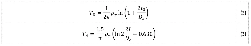
where:
• ρT : Soil thermal conductivity
• t3 : Thickness of the serving
• Ds : external diameter of metal sheath
• L : depth of laying
• De : external diameter of cable
The relation used to describe the soil thermal conductivity as a function of moisture content, is not shown. This relationship contains a dependence on soil moisture content, porosity and quartz content which then determines the type of soil considered. This information can be derived from the MERIDA dataset.
Part 2 of this article will appear in the INMR WEEKLY TECHNICAL REVIEW of Aug 18.