This contribution to INMR by Tarik Menkad, an R&D Engineer at Integrated Engineering Software in Canada explains that a hysteresis model improves accuracy of iron loss computations in FEM simulations of electrical machines. While the Preisach scalar model and the vector Preisach-Mayergoyz model are known for their accuracy, these suffer from poor numerical performance due to expensive implementation as well as convergence issues raised in the transient analysis of problems with hysteresis.
A hysteresis model improves accuracy of iron loss computations in simulating electrical machines by the finite element method (FEM). Hysteresis models based on the Preisach scalar model and its extension, the vector Preisach-Mayergoyz model, are known for their accuracy but suffer from poor numerical performance. This is due to the expensive implementation of the classical models as well as convergence issues raised in the transient analysis of problems with hysteresis.
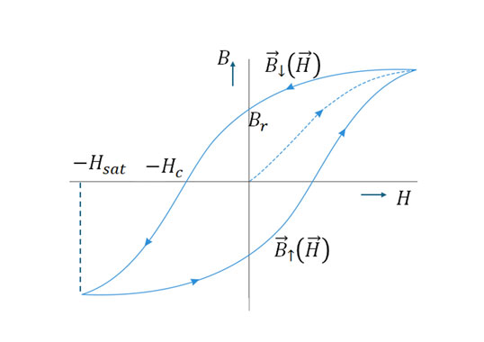
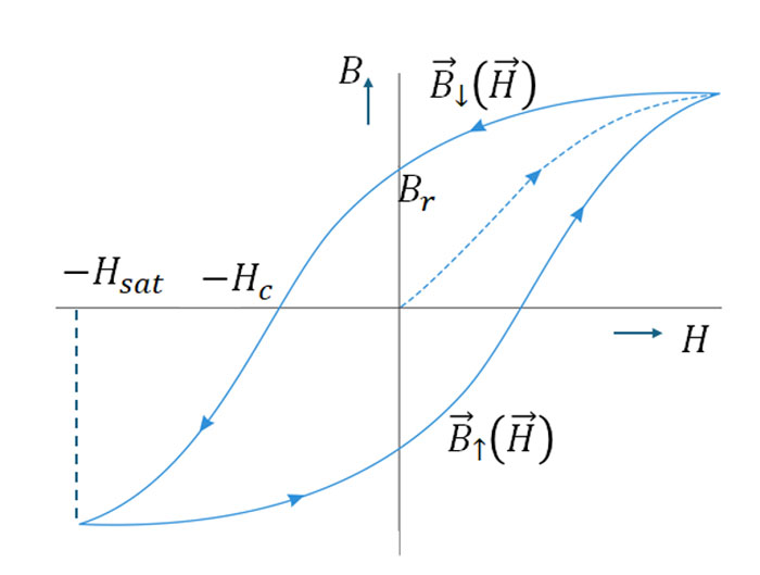
The magnetizing process in magnetic materials is a complex phenomenon. Locally, at the macroscopic scale, the thermodynamic irreversibility of the magnetization process results in a phenomenon called magnetic hysteresis. This phenomenon is usually represented in the form of a B-H curve, which corresponds to the response of a magnetic material subjected to uniaxial excitation.
From experiments, it has been observed that B-H curve possesses the following properties:
1. Relationship between B and H is highly non-linear;
2. Value of B depends not only on H but also on its history;
3. A branch occurs in the B-H curve when the value of H reaches a local extremum. This cusp is characterized by a discontinuity in the derivative of the curve;
4. Periodic variation of H oscillating between two constant values describes a closed hysteresis cycle or loop;
5. A closed and centered hysteresis cycle is symmetrical. This symmetry between the ascending branch ↑ and the descending branch ↓ is such that:
B↓ (H)=-B↑ (-H)
It is important to note that, in general, the magnetic properties of materials also depend on the direction of the applied magnetic field (anisotropy).
Certain characteristic quantities of a magnetic material are defined from its largest closed hysteresis cycle (major loop). The coercive field Hc: B↑ (Hc )=B↓ (-Hc )=0, the remanence magnetization Br: Br =B↓ (0)=-B↑ (0), and finally Bsat corresponds to the saturation magnetization (see Fig. 1). It is important to note that while both Hc and Br are defined univocally, this is not the case for Bsat.

Preisach Model
Preisach’s intuition consists in imagining that magnetic material is made up of a multitude of elementary magnetic particles called hysterons. These can take a magnetization value of +1 or −1 (in arbitrary units) and oppose a certain resistance to the change of magnetization. A hysteron Υ (β,α) is a delayed relay with a pair of thresholds (β,α), β≤α defined for a time-domain input function H(t), t∈[0,T] as
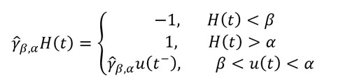
where t^-=lim(ε>0,ε→0) t-ε and γ (β,α) H(0- )∈{-1,1} is a defined initial state, see Figure II.1, and β=-α if our hysteron is isolated. However, because the magnetic particles interact with each other in a material, the effective field perceived by some hysterons must be offset from the applied magnetic field i.e. α+β≠0. The irreversible component Mirr (H) of the magnetization in the material at time t is the sum of all the contributions from hysterons.
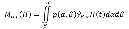
The Preisach density function p(α,β) satisfies p(-β,-α)=p(α,β) since hysterons must exist in pairs. The scalar Preisach hysteresis model possesses a geometric interpretation. In a semi plan α≥β with a limit point (α0,β0 ), β0=-α0, the stairway frontier that separates the region where all hysterons are on positive saturation (+1) from the region where the remaining ones are all on negative saturation (-1), represents the internal state of the Preisach model.
Now, to obtain a vector Preisach model, it suffices to combine the infinitesimal contributions coming from an infinity of scalar Preisach operators distributed in all possible orientations. For each of the scalar Preisach operators, the input variable corresponds to the projection of the magnetic field in this orientation.
Next, issues are examined that render the scalar Preisach and hence its vector counterpart computationally inefficient and we propose measures to address these issues.
A. Shortcoming of Classical Scalar Preisach Model
• To perform transient FEM analysis, it is common to initialize fields H and B to zero value. This corresponds to initializing the hysteresis model in the demagnetized state. Such state is poorly defined in the classical Preisach model.
• The Preisach model provides the irreversible component of the magnetization. The missing reversible component, which is an odd function with respect to the magnetic field, is therefore not represented.
B. Proposed Improvements of Scalar Preisach Model
• A perfectly demagnetized state can be approached by a diagonal Preisach boundary. This can be produced by an alternating field of amplitude initially equal to Hsat which decreases infinitely slowly towards zero. Hence it requires a lot of memory space. It proposed to redefine coordinate (α0,β0 ) as follows:
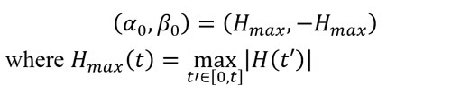
i.e. the maximum value of the amplitude of the magnetic field reached since the start of the simulation.
• To the classical model is added a reversible magnetization component Mrev which allows expressing the total magnetization as:
M(H)=Mrev (H)+Mirr (H)
Such that mapping Mrev is bijective and has odd symmetry.

Numerical Experiments
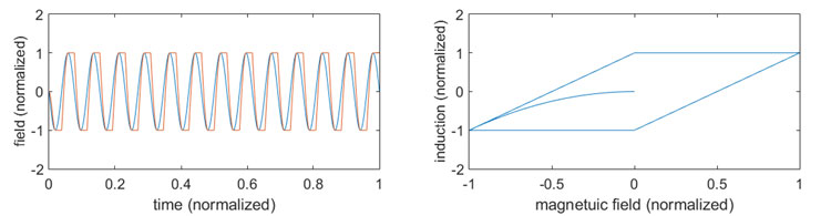
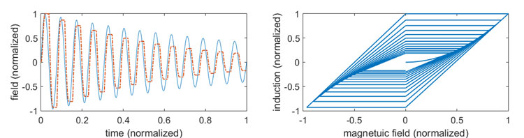
To show the correctness of the modified scalar Preisach hysteresis model, we compute the output of its constitutive relation B(H) for different input time-domain H waveforms. Fig. 2. shows the time delay between induction B and sinusoidal input field H. It also shows the hysteresis curve of the scalar Preisach model B(H). In the same way, Fig. 3 pictures the case of an exponentially decayed sinusoidal input field.
Right: Hysteresis curve B(H).
Right: Hysteresis curve B(H).
Now, the EFG-3N method is used to calculate the parameters (a_i,b_i,c_i )_(1≤i≤3) of the 2D vector Preisach model for steel 4340. A 2D uniformly rotating vector field H ⃗ of angular velocity f=10Hz is produced, with components H_x and H_y(see Fig. 4). The rotational symmetry property of the 2-D vector Preisach asserts that induction B ⃗ must also be a uniformly rotating vector field of same angular velocity, see Fig. 4. This fundamental property is satisfied by our modified Preisach hysteresis model. Finally, Fig. 4 shows the corresponding hysteresis curve along x-axis.
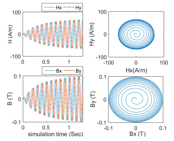
Right: x-y correspondence.
Conclusions
The scalar Preisach hysteresis model and its vector counterpart have been introduced. Through modifications, these models have been rendered attractive for their integration in 2-D and 3-D FEM solvers.